The simplest neural network consists of only one "neuron". The so-called neural network is to connect many single "neurons" together, so that the output of one "neuron" can be another "neuron". enter.
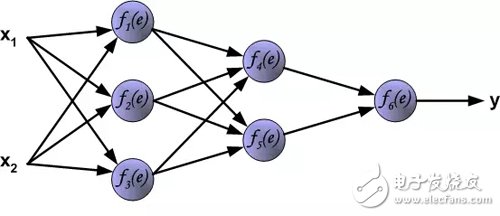
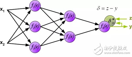
The article describes the learning process of training multi-layer neural networks using backpropagation algorithms. To illustrate this process, a three-layer neural network with two inputs and one output is used, as shown in the following figure:
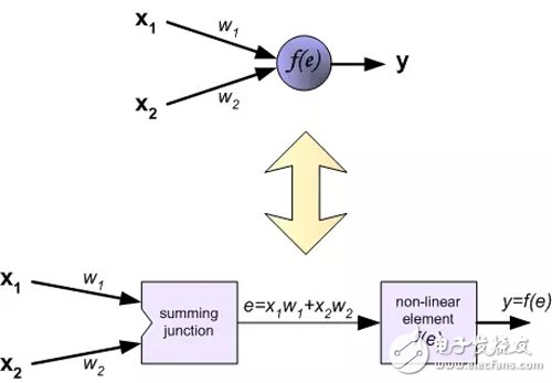
Each neuron consists of two parts. The first part is the weighted sum of the input signal and the weighting factor. The second part is a nonlinear function called a neuron activation function. Signal e is the weighted sum output (the output of the adder) signal. y=f(e) is the output signal of the nonlinear function (element). Signal y is also the output signal of the neuron.
To train a neural network, we need to "train the data set." The training data set is composed of input signals (x_1 and x_2) corresponding to the target z (expected output). The training of neural networks is an iterative process. In each iteration, the weighting coefficients of the network nodes are modified using new data from the training data set. The entire iteration consists of two processes, forward calculation and back propagation.
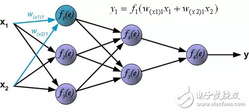
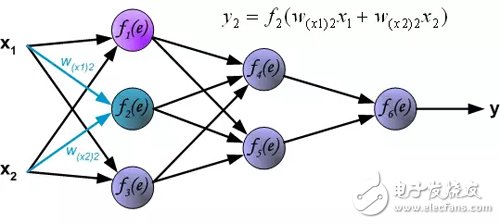
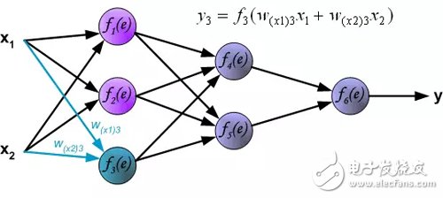
Forward calculation: Each learning step begins with two input signals from the training set. After the forward calculation is complete, we can determine the output signal value of each neuron in each layer of the network (Translator's Note: the error of the hidden layer neurons is not available, because there is no hidden layer target value in the training data set). The figure below shows how the signal propagates through the network, and the symbol w(xm) represents the connection weight between the network input x_m and the neuron n. The symbol y_n represents the output signal of the neuron n.
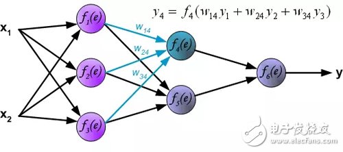
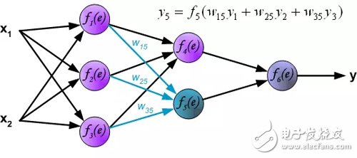
Hidden layer signal propagation. The symbol w_mn represents the connection weight between the output of the neuron m and the input of the next layer of neuron n.
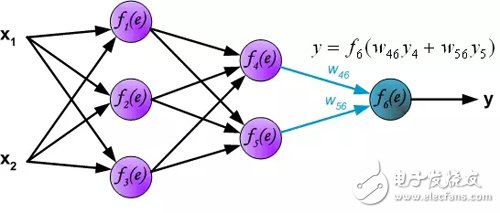
Output layer signal propagation:
In the next algorithm step, the output signal of network y is compared to the output value (target) in the training data set. The difference is called the error signal δ of the output layer neurons.
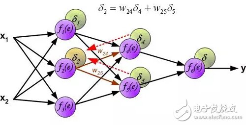
Since the output value of the hidden layer neurons (the training set has no target value of the hidden layer) is unknown, it is impossible to directly calculate the error signal of the internal neurons. Over the years, there has been no effective way to train multi-layer neural networks. Until the mid-eighties, backpropagation algorithms were developed. The backpropagation algorithm propagates the error signal δ (calculated in a single training step) back to all neurons, and for neurons, the error signal propagates back.
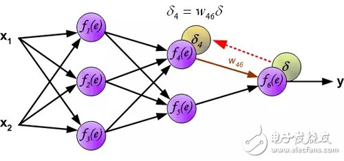
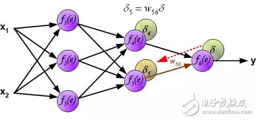
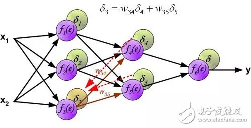
The weighting factor w_mn for the propagation error is equal to the weighting factor used for the forward calculation, except that the direction of the data stream changes (the signal propagates one by one from the output to the input). This technique is used for all network layers. If the error is from multiple neurons, add them up. (Translator's Note: In the reverse direction, it is also a weighted sum). The figure below shows:
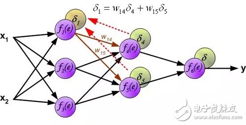
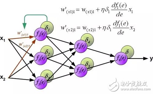
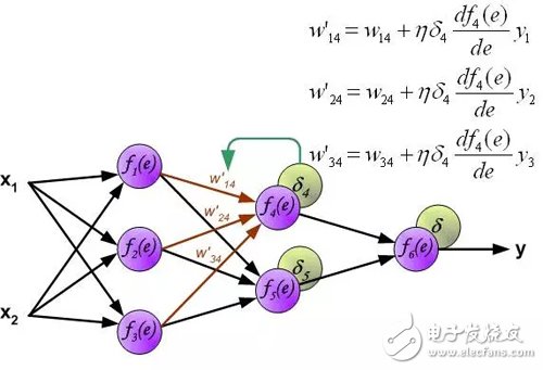
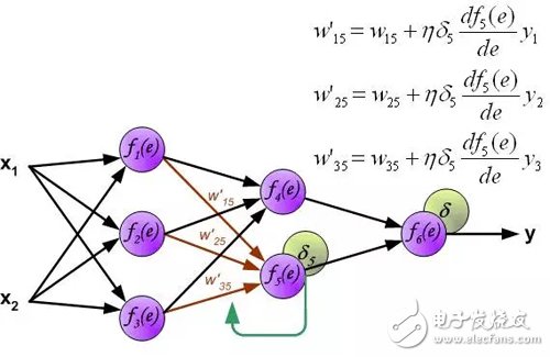
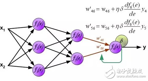
An error signal for each neuron is calculated for modifying the weighting coefficients for each neuron input connection. In the formula below, df(e)/de represents the derivative of the neuron activation function. In addition to the derivative of the neuron activation function, the factors affecting the weight also have an error signal for back propagation and the previous neuron connected by the direction of input of the neuron. (Translator's Note: Ignore the derivation process here, directly give the weight modification method. The specific derivation process refers to my previous article: "Error backpropagation algorithm shallow solution." The principle is the same, affecting the weight of three The factors are reflected in the formula below.).
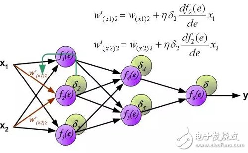
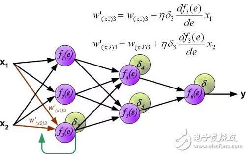
The coefficient η affects the network training speed. There are several techniques to choose this parameter. The first method is to start with a larger parameter value. When the weighting factor is being established, the parameters are gradually reduced. The second method is to start training with small parameter values. During the training process, the parameters gradually increase and then fall again in the final stage. Starting a training process with low parameter values ​​can determine the weighting factor.
There are many different versions of DIN Connectors. The name of each type comes from the number of pins the connector has (3-pin DIN, 4-pin DIN, etc.) Some of these pin numbers come in different configurations, with the pins arranged differently from one configuration to the next.
DIN cable connector 3-pin, 4-pin, 5-pin, 6-pin, 7-pin, 8-pin degree 180, 216, 240, 262, 270
DIN cables, DIN connector, telephone cable, computer cable, audio cable
ETOP WIREHARNESS LIMITED , https://www.wireharness-assembling.com